
LESSON 13: INDUSTRIAL GROWTH CURVES
If one attempts to follow the industrial development that has taken place in the Western World since the year 1700 by attempting to take into account all of the separate inventions and technical developments that have occurred in the various fields of industry, he soon finds himself hopelessly involved. Order, however, readily emerges from this chaos when one considers that all of this industrial activity has been based in the main upon the use of a few relatively simple substances, chiefly, the few industrial metals—iron, copper, tin, lead, zinc, etc.—as the essential materials for machinery, and the use of a few basic sources of energy, chiefly, the mineral fuels, coal, oil and natural gas, and, of lesser importance, water power.
The most accurate quantitative picture of the rate and magnitude of our industrial growth, however, could be obtained by plotting growth curves of the production of these primary metals and of energy. In this lesson we are presenting, therefore, the growth curves of a number of our basic industries—the production of pig iron, coal, energy, railroads, and automobiles. These curves are plotted with the vertical dimension representing the quantity produced per annum, the horizontal dimension measured from left to right representing time in years.*
Pig Iron. There are a number of highly instructive details to be observed about each of these curves. In the first case, they are not smooth, but are, instead, jagged or zig-zag. This is due to the fact that the production fluctuated from one year to the next. This is particularly noticeable in the case of pig iron.
* The data for these curves were obtained from the Mineral Resources of the U.S.A., U.S. Statistical Abstracts and Mineral Industry, Vol. 41. For 1933 figures the Survey of Current Business was used. These volumes contain the most authoritative figures that can be obtained.
In Figure 1 notice the drop in the production of pig iron during the depression of 1893 and 1894 and, after that depression, notice that the pig iron industry expanded for a number of years, and enjoyed uninterrupted prosperity.
Then came the depression of 1908, which shows up as a severe shutdown in the pig iron industry. This shutdown lasted one year, followed by a still further expansion and growth culminating in the large peak of production from 1916 to 1918, showing the effect of large war orders for steel.
Note next the depression of 1921. After this the pig iron industry recovered somewhat, but did not expand as rapidly. The highest peak of production in pig iron was reached in 1929. This was followed immediately by the enormous drop due to the present depression. [1932-33]
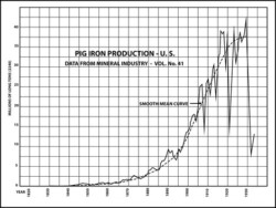
Figure 1
What were the actual magnitudes of these depressions? If we measure the graph, we find that the drop in production from peak to trough in 1893 and 1894 was 27 percent; in 1908 the corresponding drop was 38 percent; in the depression of 1921, the shutdown in pig iron was 57 percent from the previous peak of production; the drop since 1929 has been 79 percent. [to 1933]
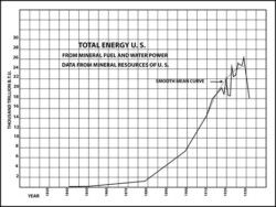
Figure 2
What does this mean? Simply this: that, stated in terms of physical measurements, each depression since 1894 has been progressively bigger than the previous. These up and down movements of the production curve are spoken of as swings or oscillations. The biggest oscillations since 1893-94 coincide with the financial depressions. Each one of these depression oscillations has had an amplitude or depth of swing approximately 30 percent greater than the one preceding. If one examines the other curves, that of coal, for instance, or of automobiles, he finds a similar situation. The larger the production becomes the larger become the oscillations; the largest being in each case that since 1929, both in absolute magnitude and also in percentage of the total production. (The smooth part of the total energy graph [Figure 2] for the time preceding 1918 does not indicate that there were no oscillations in this period in energy production because in this part of the graph the figures are all averaged for ten-year periods. This method of plotting smooths out the oscillations.)
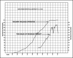
Figure 3
Growth of railroads. Figure 3 shows no oscillations because it represents the number of miles of railroad track in operation and this, of course, increases, but rarely decreases, from year to year. The oscillations of exactly the same kind as those exhibited by pig-iron, however, are found in the second railroad graph, that of ton-miles of revenue freight hauled. (One ton-mile is equal to one ton hauled one mile.)
Point of Inflection. Another feature to be observed about each of these growth curves is that represented by the smooth dotted-line curve. This dotted-line curve has in each case been drawn to represent the mean rate of growth. Notice in each case the S-shape of this curve. In the beginning it starts up very gradually, but each year the increase in production is greater than that for the year preceding and during this time period the curve is concave upward. Finally, in each case there comes a time when the growth begins to slacken, and the curve becomes convex upward and begins to level off rapidly. The point at which this smooth mean curve changes from concave upward to convex upward is called the point of inflection.
This point of inflection occurred in pig iron about the year 1905; in railroad trackage about 1885; in railroad freight haulage about 1910; in automobile production about 1921, and in ‘all energy’ about 1912.
Calculation shows that the state of growth before the point of inflection is reached has been a compound interest rate of growth; that is to say, that the production each year during that period was on the average a certain fixed percentage greater than that of the year before. In the case of coal and energy production this rate of increase was approximately 7 percent per annum during that same period. The same is true for pig iron. In other words, with the rate of growth that prevailed during that period the annual production was increased tenfold in 321/2 years.
All of the graphs mentioned thus far have been those of basic industries, extending back approximately a hundred years or more. Since not infrequently our economic soothsayers assure us that as older industries reach their saturation, or decline, newer and bigger industries always rise to take their places, it becomes a matter of some particular importance to examine the rise in growth of one of these newer industries. Of such industries, automobiles are by far the most striking example. The automobile industry practically began in the year 1900. Since that time it has risen into one of the greatest of our present industries, and has practically revolutionized our social life in the process.
Production of Automobiles. In what manner did the production of automobiles grow? A glance at the growth of automobile production in Figure 4 will indicate that the production of automobiles grew in a manner essentially similar to those older industries we have just discussed. In this curve, just as in those previous, there are zig-zag oscillations, by far the greatest being that since 1929.
The production of automobiles reached an all-time peak in the year 1929, with an annual production of 5,600,000 automobiles. From that time until 1932 the production dropped to 1,400,000 cars per annum, a shut-down of 75 percent. A mean curve of this growth of automobile production shows a distinct leveling-off since the year 1923. The point of inflection of the mean growth curve occurs about the year 1921-22. The broken line curve on the Automobile chart represents the number of registered motor vehicles in the United States. It will be noted that this number in 1929 was something over 26,000,000. Also notice that this curve has been leveling off since 1926.
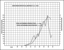
Figure 4
Radio. Or, to select another new industry, radio is an excellent example. Unfortunately, reliable data are not available for plotting a growth curve of the number of radio sets. This much, however, we do know, that radio broadcasting began on a commercial scale about the year 1921. From that time it grew with amazing rapidity until by 1929 by far the greater number of people in this country had radio sets. Since that time the number of radio sets in operation appears, from such data as are available, to be increasing but slightly.
Biological Growth Curves. From the study of the foregoing graphs of the growths of various of our basic industries the persistent S-shape of each of the growth curves examined is a striking and singular phenomenon, and merits further investigation.
Dr. Raymond Pearl, in his book, Biology of Population Growth, has made an extensive study of types of growth, and has found that almost every growth phenomenon exhibits this same S-shape characteristic. One of his experiments consisted in placing a pair of fruit flies in a bottle, and letting them multiply while he kept a record of the increase of the fly population on successive days. When plotted as a growth curve after the manner of the charts above, the curve of the growth of the fly population would be indistinguishable from our mean curve of coal or pig iron production.
Bacteriologists have found that yeast cells or bacteria when placed in a test tube under conditions favorable for their multiplication increase in numbers in a manner identical to that discussed above. Dr. Pearl has found ample evidence that human populations obey the same laws of growth.
Fallacy of Economists. It is a simple matter to see why in the initial stages organisms and new industries should, under favorable conditions, expand at approximately a compound interest rate of growth. Since, until recently, most of the industrial development of this country has still remained in the compound interest stage, it has come to be naively expected by our business men and their apologists, the economists, that such a rate of growth was somehow inherent in the industrial processes. This naive assumption was embodied in the graphs and charts made by these gentlemen, in which ‘normal’ conditions were taken to be a steady industrial growth at the rate of 5 percent or more per annum. Such conditions being ‘normal,’ it was further assumed, without question, that such normal growth would continue indefinitely. We have already seen that the actual facts warrant no such assumption.
The question remains, however, as to why these growth processes have abandoned the original upward trend and tend to level off or reach a stage of saturation. The simplest case, perhaps, with which to answer this question would be that of the growth of fruit flies inside their bottle universe. Should the fruit flies continue to multiply at their initial compound interest rate, it can be shown by computation that in a relatively few weeks the number would be considerably greater than the capacity of the bottle. This being so, it is a very simple matter to see why there is a definite limit to the number of fruit flies that can live in the bottle. Once this number is reached, the death rate is equal to the birth rate, and population growth ceases.
Very little thought and examination of the facts should suffice to convince one that in the case of the production of coal, pig iron or automobiles, the circumstances are not essentially different.
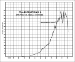
Figure 5
Coal. As we have pointed out already, during the period from 1860 to 1910 coal production increased at the rate of 7 percent per annum. According to the report of the International Geological Congress in 1912, the coal reserves of the United States are about 3.8 million tons (3.8×10¹² tons). Had our rate of coal consumption continued to grow at 7 percent per annum, all the coal reserves of the United States would be exhausted by the year 2033, almost exactly 100 years hence.
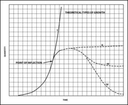
Figure 6
Theoretical Growth Curves. The exhaustion of coal or of any other mineral resource is, however, not something that happens suddenly, but occurs very gradually instead, by a process which is somewhat analogous to the dipping of water from a pail, when one is allowed to take only one-tenth of what remains each time.
To show the various types of growth a chart of four theoretical growth curves has been inserted.
In Figure 6, Curve I represents pure compound interest at 5 percent per annum. It will be noticed that many physical types of growth approximate this curve in its lower parts, but ultimately, due to the fact that no physical quantity can increase indefinitely, all cases of physical growth must depart from this initial compound interest curve. The later stages in various types of physical growth are shown in Curves II, III and IV.
Curve II represents a type of growth which reaches a maximum, and thereafter remains constant. A familiar illustration of this type of growth is represented by water power. Power produced from waterfalls in a given area can increase until all the falls are harnessed. Thereafter, provided the installations are maintained, the production of such power remains constant.
Curve III represents a type of growth which reaches a maximum, then declines somewhat, and finally tends to level off at some intermediate level. In the United States the production of lumber follows such a curve as III. In the initial conditions virgin timber was slashed off, and the lumber industry grew until it reached a production peak. Then, as the forests diminished, the production of lumber tended to decline. The final leveling-off process will be reached when the production of lumber shall be maintained equal to the rate of growth of forests and reforestation.
Curve IV is the type of growth curve characteristic of the exploitation of any non-recurrent material, such as all mineral resources. Coal, oil and the metals all exist in minable deposits in definitely limited quantities. One of the simplest illustrations of a curve such as type IV is illustrated in the life history of a single oil pool. In an oil pool the production rises as more and more wells are drilled, until it reaches a peak. From that time on the production declines year by year, until finally it becomes so small that the pool is abandoned. In most American oil pools the greater part of this history takes place within 5 to 8 years after the discovery, though the pool may continue to be operated for the small remaining amount of oil for 10 or 15 years longer.
In the case of mineral fuel, such as coal and oil, it is the energy content that is of importance in use. This energy is degraded in accordance with the second law of thermodynamics. Thus, coal and oil can only be used once. The case of the metals is somewhat different. Iron, copper, tin, lead, zinc, etc., can be used over and over again, and are never in a physical sense destroyed. In the process of using metals, however, there is a continuous wastage through oxidation and other chemical reactions, through the discarding of iron and tin in the form of tin cans, razor blades, etc. While this does not destroy the metal it disseminates it in such a manner as to render it unavailable for future use.
Primary metals are derived from naturally occurring ore deposits containing the metallic salts and other compounds at relatively high concentrations. Thus, there is a flow of metals from the limited deposits at high concentrations into industrial uses, and finally, by wastage and dissemination, back to earth again in widely scattered and hence unavailable forms. This process, like that of the degradation of energy, is unidirectional and irreversible. It follows, therefore, that the production of the rarer metals, such as are now most commonly used in industrial processes, must ultimately reach its peak and decline after the manner illustrated by Curve IV.
It is not intended to convey by the above calculations the impression that the leveling-off of our present growth curves is due as yet in any large measure to exhaustion or scarcity of resources. The resource limitations are cited only as an illustration of one of the many things that must eventually aid in producing this result.
Social and Industrial Results. The leveling-off of the production curves thus far has been due largely to a saturation in the ability to consume under our existing Price System limitations of the ability of the individual to purchase. There is a definite limit as to how much food an individual can consume in a given time; how many clothes he can wear out; and, in general, how much energy degradation he can account for. There is no question but that in many respects the people of the United States prior to 1929 were approaching some of these limits, and that accounts in some degree for the slowing down of the growth of production in many fields. There was an average at that time of one automobile per family. This fact, together with the consequent congestion of traffic, was sufficient to depress the rate of growth of automobile production.
Another important factor that is rarely taken into account in this connection is that, due to the change of rate in the operation of physical equipment, at the present time almost every new piece of machinery runs faster than the obsolete one which it displaces. There is a physical relationship in all physical equipment to the effect that for a given rate of output the faster machinery is made to operate, the smaller it needs to be. Compare, for example, the size of a 1 h.p. high-speed electric motor with a slow-acting gasoline engine of the same power. This relationship is true, whether the equipment be individual machines, whether it be a whole factory, or whether it be a whole industry. Since the production of consumable goods is leveling off, and the machinery is being continuously sped up, it follows that our industrial plants and equipment, instead of getting larger, may actually diminish in size.
The implication of this fact with regard to the demand for such raw materials as iron, copper, etc., is far-reaching. In our pioneer days, and during the period of most rapid growth, railroads, telegraph and telephone systems, power systems, and factories, had to be built, each requiring its quota of primary metals. Now that these things have already been built, the materials for the construction of new equipment are largely obtained by junking the equipment now obsolete. To appreciate the importance of this rise in the use of secondary metals, consider the fact that in the year 1933 the production of secondary copper was over 90 percent of that of the primary copper in the United States for that year.
Summary
In this lesson we have tried to show in quantitative terms what the leading facts of our industrial expansion have been. Man’s learning to convert to his own uses the vast supply of energy contained in fossil fuels—coal and oil—has opened up a totally new and unparalleled phase of human history. It has been estimated that the effect of this upon the biological equilibrium of the human species has been such that the human population on the globe has approximately tripled since the year 1800. Areas like the British Isles, which, under a pre-technological state of the industrial arts, were able to support only from 5,000,000 to 8,000,000 people, now have populations of approximately 46,000,000, or a population density of 490 persons per square mile.
It has been shown that this industrial growth has been characterized in the initial stages by a compound interest rate of expansion of about 7 percent per annum in the United States. It has also been shown that not only is it impossible to maintain for more than a few decades such a rate of expansion, but that in the United States that period of most rapid growth has passed, and that already more or less unconsciously we have entered well into the second period of growth, that of leveling off and maturation.
Due to the physical limitations it seems at present that the days of great industrial expansion in America are over unless new and as yet untapped sources of energy become available. We have been told repeatedly that new industries have been and will continue to be sufficient to maintain the industrial growth as older industries slacken. Consideration of the graph of total energy which represents the motive power of all industries, new and old, indicates that, until the present, such has not been the case, and there are no prospects that it will be so in the future.
Foreign trade has been frequently invoked as a means of maintaining our industrial growth. Invariably in such cases, however, foreign trade has been discussed implicitly as a ‘favorable balance of trade,’ which implied that the amount exported will be in excess of the amount imported. Physically a ‘favorable balance of trade’ consists in shipping out more goods than we receive. Following this logic a ‘perfect trade balance’ should consist in a state of commerce wherein everything was shipped out and nothing received in return.
Under our present Price System, or monetary economy, an unbalanced foreign trade can only be maintained, as we are learning to our sorrow, for a comparatively short length of time. With a balance of trade there is no reason to expect any essential increase in the domestic production of this country by means of foreign markets for such a condition necessitates that approximately equal quantities of goods be obtained from abroad, and the net effect is zero.
References:
- S. Minerals Yearbook.
- World Minerals and World Politics, Leith.
- Man and Metals, Rickard.
- Mineral Raw Materials, Bureau of Mines Staff.
- Mineral Economics, Tryon and Eckel. Minerals in Modern Industry, Voskuil.
- Statistical Abstract of the U.S.